ESA Digital Twin Earth (DTE) Framework
A common grid for Earth Observation and climate data
GRID4EARTH builds a unified, standardized data infrastructure on Discrete Global Grid Systems — ellipsoidal HEALPix — so Copernicus Sentinel and Destination Earth data become analysis-ready, interoperable, and cloud-native.
One grid to bridge models and observations
Copernicus and Destination Earth produce massive global datasets on heterogeneous grids — regular lat/lon, reduced Gaussian, swath geometries, unstructured meshes. Reconciling them means ad-hoc regridding that is costly, error-prone, and not reproducible. GRID4EARTH adopts a single Discrete Global Grid System (DGGS) — the HEALPix equal-area grid, referenced to the WGS84 ellipsoid — combined with cloud-optimized Zarr V3 storage, so data from every mission shares one analysis-ready surface.
Equal area at every depth
HEALPix nested is a native quadtree: each pixel subdivides into four children with identical surface area at any resolution — unbiased statistics and trivial up/downscaling.
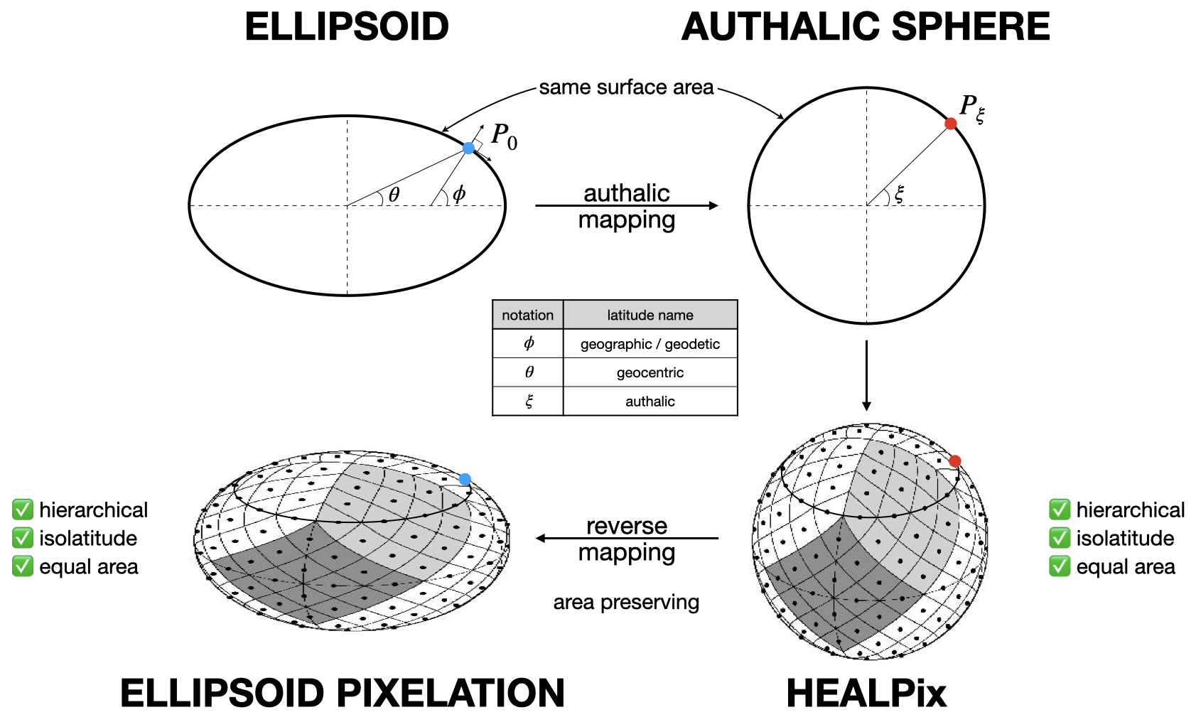
Ellipsoidal, not just spherical
HEALPix is defined on a sphere, but Earth is a WGS84 ellipsoid. At Copernicus resolution that 0.3% flattening matters. An authalic-sphere mapping preserves equal area on the ellipsoid.
Cloud-native & AI-ready
Space-filling-curve locality maps to GPU batches and ML-friendly tiles; quadtree nodes align with Zarr / COG chunks for scalable object-store access.
From a fragmented grid landscape to analysis-ready data
HEALPix gives climate models (on the sphere) and Earth Observation (on the ellipsoid) a single common grid — no regridding, consistent statistics, interoperable workflows.
Show the code for this figure
"""Interactive HEALPix globe (Plotly) for the GRID4EARTH homepage.

Reproduces the GRID4EARTH BIDS25_demo / dggs_intro globe: a rotatable dark 3D
globe with the HEALPix grid (NESTED), the cell-ID numbers at each cell centre,
coastlines, and hover that reports lon/lat. Writes a standalone HTML embed to
static/embeds/healpix-globe.html (Plotly.js from CDN).

Deps: plotly, healpy, numpy.  Coastlines come from a Natural Earth 110m GeoJSON
fetched at build time — no cartopy needed.

Usage:
    pip install plotly healpy numpy
    python scripts/figures/make_healpix_globe.py
"""

import json
import urllib.request
from pathlib import Path

import healpy as hp
import numpy as np
import plotly.graph_objects as go

OUT = Path(__file__).resolve().parents[2] / "static" / "embeds"
COAST_URL = (
    "https://raw.githubusercontent.com/nvkelso/natural-earth-vector/"
    "master/geojson/ne_110m_coastline.geojson"
)

NSIDE = 2            # refinement level 1 -> 48 cells (matches the demo)
RED = "#e8392a"     # HEALPix grid + cell-id labels
CYAN = "#00b5e2"    # coastlines


def sph2cart(lon, lat, r=1.0):
    lon, lat = np.radians(lon), np.radians(lat)
    return (
        r * np.cos(lat) * np.cos(lon),
        r * np.cos(lat) * np.sin(lon),
        r * np.sin(lat),
    )


def healpix_grid_trace(r=1.005):
    """All NESTED cell boundaries at NSIDE as one red Scatter3d (NaN-separated)."""
    xs, ys, zs = [], [], []
    for pix in range(hp.nside2npix(NSIDE)):
        x, y, z = hp.boundaries(NSIDE, pix, step=24, nest=True)
        xs += [*(r * x), r * x[0], np.nan]
        ys += [*(r * y), r * y[0], np.nan]
        zs += [*(r * z), r * z[0], np.nan]
    return go.Scatter3d(x=xs, y=ys, z=zs, mode="lines",
                        line=dict(color=RED, width=2), hoverinfo="skip", showlegend=False)


def cell_label_trace(r=1.01):
    """Cell-id numbers at each cell centre; hover shows the cell id + lon/lat.
    Centres sit on the globe so the opaque surface hides the back-facing labels."""
    ipix = np.arange(hp.nside2npix(NSIDE))
    lon, lat = hp.pix2ang(NSIDE, ipix, nest=True, lonlat=True)
    x, y, z = sph2cart(lon, lat, r=r)
    lon = ((lon + 180) % 360) - 180
    return go.Scatter3d(
        x=x, y=y, z=z, mode="text", text=[str(p) for p in ipix],
        textfont=dict(color=RED, size=12), showlegend=False,
        customdata=np.column_stack([ipix, lon, lat]),
        hovertemplate="cell %{customdata[0]}<br>lon %{customdata[1]:.1f}°, lat %{customdata[2]:.1f}°<extra></extra>",
    )


def coastline_trace(r=1.004):
    try:
        with urllib.request.urlopen(COAST_URL, timeout=60) as resp:
            data = json.loads(resp.read())
    except Exception as exc:
        print("WARNING: could not fetch coastlines:", exc)
        return None
    xs, ys, zs = [], [], []

    def add(coords):
        coords = np.asarray(coords)
        if coords.ndim != 2 or coords.shape[0] < 2:
            return
        x, y, z = sph2cart(coords[:, 0], coords[:, 1], r=r)
        xs.extend([*x, np.nan]); ys.extend([*y, np.nan]); zs.extend([*z, np.nan])

    for feat in data["features"]:
        geom = feat["geometry"]
        if geom["type"] == "LineString":
            add(geom["coordinates"])
        elif geom["type"] == "MultiLineString":
            for line in geom["coordinates"]:
                add(line)
    return go.Scatter3d(x=xs, y=ys, z=zs, mode="lines",
                        line=dict(color=CYAN, width=2), hoverinfo="skip", showlegend=False)


def build():
    fig = go.Figure()

    # dark globe surface; hover anywhere reports lon/lat
    u = np.linspace(0, 2 * np.pi, 120)
    v = np.linspace(0, np.pi, 120)
    R = 0.99
    xs = R * np.outer(np.cos(u), np.sin(v))
    ys = R * np.outer(np.sin(u), np.sin(v))
    zs = R * np.outer(np.ones_like(u), np.cos(v))
    lon2d = (np.degrees(u)[:, None] + 180) % 360 - 180
    lat2d = 90 - np.degrees(v)[None, :]
    custom = np.dstack([np.broadcast_to(lon2d, xs.shape), np.broadcast_to(lat2d, xs.shape)])
    fig.add_trace(go.Surface(
        x=xs, y=ys, z=zs, showscale=False,
        colorscale=[[0, "rgb(64,64,64)"], [1, "rgb(22,22,22)"]],
        lighting=dict(ambient=1, diffuse=0, specular=0),
        customdata=custom,
        hovertemplate="lon %{customdata[0]:.1f}°, lat %{customdata[1]:.1f}°<extra></extra>",
    ))

    fig.add_trace(healpix_grid_trace())
    coast = coastline_trace()
    if coast is not None:
        fig.add_trace(coast)
    fig.add_trace(cell_label_trace())

    fig.update_layout(
        scene=dict(
            xaxis=dict(visible=False), yaxis=dict(visible=False), zaxis=dict(visible=False),
            aspectmode="data", bgcolor="rgba(0,0,0,0)",
            camera=dict(eye=dict(x=1.25, y=1.25, z=0.85)),
        ),
        paper_bgcolor="rgba(0,0,0,0)",
        margin=dict(l=0, r=0, t=0, b=0),
        showlegend=False,
    )
    return fig


if __name__ == "__main__":
    OUT.mkdir(parents=True, exist_ok=True)
    out = OUT / "healpix-globe.html"
    build().write_html(
        out, include_plotlyjs="cdn", full_html=True,
        config={"displayModeBar": False, "responsive": True},
    )
    print("wrote", out)
The problem
Every dataset lives on a different grid. Users repeat ad-hoc interpolations, lose information to aliasing and area bias, and get different results per workflow. There is no shared standard.
The candidate
HEALPix — Hierarchical Equal Area isoLatitude Pixelisation. Already adopted by DestinE's Climate Digital Twin, ECMWF, Planck, WMAP and Euclid. A native quadtree with equal-area cells and iso-latitude rings.
The GRID4EARTH path
Ellipsoidal HEALPix via the authalic sphere: an exact, invertible, area-preserving mapping that keeps the equal-area guarantee on WGS84. Backward compatible with standard HEALPix — only the coordinate mapping changes, no new tooling.
How healpix-geo keeps equal area on the real Earth
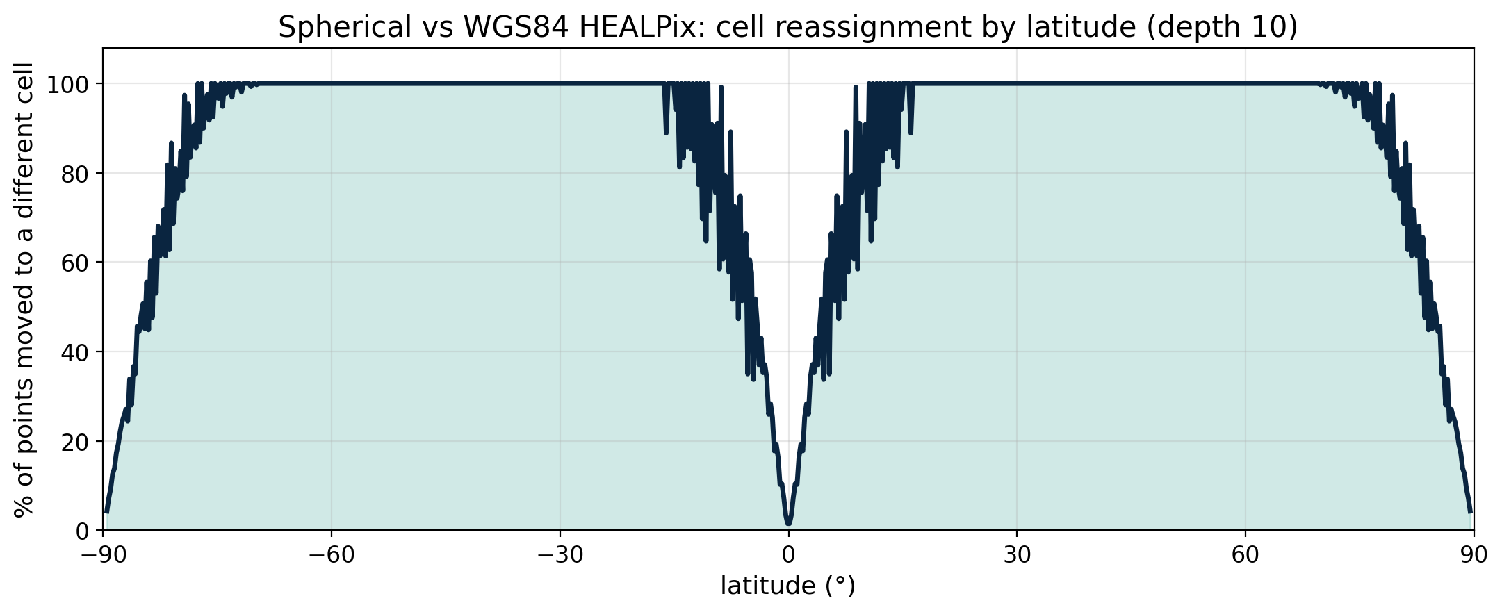
HEALPix is defined on a perfect sphere — but Earth is a WGS84 ellipsoid. At Copernicus resolution that ~0.3% flattening introduces a latitude-dependent area bias of up to 0.67%, enough to break zonal statistics. healpix-geo maps the ellipsoid onto an authalic (equal-area) sphere, pixelises it with standard HEALPix, then maps back. The transform is exact, invertible to ~1 nm, and backward compatible with spherical HEALPix — only the coordinate mapping changes, so no new tooling is needed.
import numpy as np
import healpix_geo.nested as hpx

lon = np.array([2.35, -74.0])    # Paris, New York
lat = np.array([48.85, 40.71])

# HEALPix cell ids on the WGS84 ellipsoid — not a sphere
cells = hpx.lonlat_to_healpix(lon, lat, depth=12, ellipsoid="WGS84")

parents = cells >> 2             # O(1) hierarchical refinement
Evaluate HEALPix on the WGS84 ellipsoid — one keyword. The sphere-vs-WGS84 comparison below is produced by this same library. View the figure code →
Why the reference surface matters
Show the code for this figure
# Extracted from scripts/figures/make_dggs_figures.py

def make_sphere_vs_ellipsoid(out="healpix-sphere-vs-ellipsoid.png", depth=10):
    """How often the reference surface (sphere vs WGS84) changes a point's HEALPix
    cell, as a function of latitude. A clean curve — no per-pixel map (which would
    alias into moiré near the poles where HEALPix cells fan out)."""
    lons = np.linspace(-180, 180, 1440)
    lats = np.linspace(-89.5, 89.5, 720)
    lon_g, lat_g = np.meshgrid(lons, lats)
    s = hpx.lonlat_to_healpix(lon_g.ravel(), lat_g.ravel(), depth, ellipsoid="sphere")
    e = hpx.lonlat_to_healpix(lon_g.ravel(), lat_g.ravel(), depth, ellipsoid="WGS84")
    frac = 100.0 * (s != e).reshape(lat_g.shape).mean(axis=1)

    fig, ax = plt.subplots(figsize=(11.0, 4.6), dpi=200)
    ax.fill_between(lats, 0, frac, color=TEAL, alpha=0.22)
    ax.plot(lats, frac, color=NAVY, lw=2.5)
    ax.set_title(f"Spherical vs WGS84 HEALPix: cell reassignment by latitude (depth {depth})")
    ax.set_xlabel("latitude (°)")
    ax.set_ylabel("% of points moved to a different cell")
    ax.set_xlim(-90, 90); ax.set_ylim(0, max(5, frac.max() * 1.08))
    ax.set_xticks([-90, -60, -30, 0, 30, 60, 90])
    ax.grid(alpha=0.3)
    ax.margins(x=0)
    fig.tight_layout()
    fig.savefig(OUT / out, bbox_inches="tight", facecolor="white")
    plt.close(fig)
    print("wrote", out, f"(max {frac.max():.1f}% reassigned)")
Show the code for this figure
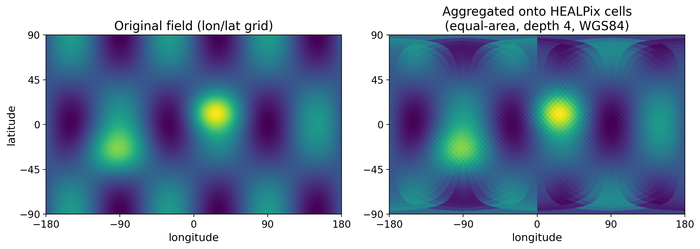
# Extracted from scripts/figures/make_dggs_figures.py

def make_data_demo(out="healpix-resample-demo.png", depth=4):
    """A continuous field aggregated onto equal-area HEALPix cells (WGS84)."""
    lons = np.linspace(-180, 180, 720)
    lats = np.linspace(-90, 90, 360)
    lon_g, lat_g = np.meshgrid(lons, lats)
    field = (
        np.sin(np.radians(3 * lon_g)) * np.cos(np.radians(2 * lat_g))
        + 1.8 * np.exp(-(((lon_g - 25) / 28) ** 2 + ((lat_g - 12) / 18) ** 2))
        + 1.4 * np.exp(-(((lon_g + 95) / 38) ** 2 + ((lat_g + 28) / 22) ** 2))
    )
    cells = hpx.lonlat_to_healpix(lon_g.ravel(), lat_g.ravel(), depth, ellipsoid="WGS84")
    _, inv = np.unique(cells, return_inverse=True)
    means = np.bincount(inv, weights=field.ravel()) / np.bincount(inv)
    aggregated = means[inv].reshape(lat_g.shape)

    fig, (a0, a1) = plt.subplots(1, 2, figsize=(12.0, 4.4), dpi=200)
    kw = dict(extent=[-180, 180, -90, 90], origin="lower", cmap="viridis", aspect="auto")
    for ax, img, title in ((a0, field, "Original field (lon/lat grid)"),
                           (a1, aggregated, f"Aggregated onto HEALPix cells\n(equal-area, depth {depth}, WGS84)")):
        ax.imshow(img, **kw)
        ax.set_title(title)
        ax.set_xticks([-180, -90, 0, 90, 180]); ax.set_yticks([-90, -45, 0, 45, 90])
        ax.set_xlabel("longitude")
    a0.set_ylabel("latitude")
    fig.tight_layout()
    fig.savefig(OUT / out, bbox_inches="tight", facecolor="white")
    plt.close(fig)
    print("wrote", out)
All four figures come from one script:
scripts/figures/make_dggs_figures.py
— reproduce with pip install -r scripts/figures/requirements.txt && python scripts/figures/make_dggs_figures.py · View on GitHub →
The HEALPix tool family
A coherent open-source stack — built by GRID4EARTH — to index, resample, analyse and plot Earth data on the HEALPix grid. All free, on PyPI / conda-forge, with WGS84 ellipsoidal support.
grid4earth
The meta-package — “pip install grid4earth” installs the whole stack at once: healpix-geo, -resample, -analyse and -plot.
healpix-geo
Core HEALPix coordinate algorithms for the geosciences, on the WGS84 ellipsoid. The foundation the rest of the stack builds on.
healpix-resample
Regrid (lon, lat) data onto a HEALPix grid with GPU-accelerated sparse operators — nearest-neighbour and PSF interpolation.
healpix-analyse
A differentiable PyTorch toolkit for analysing signals on HEALPix grids — spherical harmonics, gauge-equivariant convolution, multi-resolution.
healpix-plot
Fast, practical static plots of HEALPix data with matplotlib and cartopy, with WGS84 ellipsoidal support.
Viewers & integrations
Third-party tools that GRID4EARTH extends with HEALPix-ellipsoid support, so DGGS data works in the wider ecosystem.
xdggs
An Xarray extension for Discrete Global Grid Systems — index, select and aggregate labelled data on HEALPix, H3 and more.
Developed by the Xarray community — GRID4EARTH contributes HEALPix-ellipsoid support.
GridLook
A WebGL 3D globe viewer for HEALPix / DGGS Earth-system data — runs in the browser, loads any public Zarr dataset.
Developed by external partners — GRID4EARTH added HEALPix-ellipsoid support.
Featured examples
One worked, runnable example per GRID4EARTH tool — each showcasing a different part of the stack, from indexing to resampling to analysis to plotting.
earthcare-dggs
Convert ESA EarthCARE L2 satellite data (MSI / ATLID / CPR) to HEALPix DGGS-Zarr with healpix-geo and xdggs.
fiesta-scattering-sst-healpix-geo
Does the WGS84 ellipsoid matter for SST gap-filling? A sphere-vs-ellipsoid HEALPix comparison for scattering-transform reconstruction of Copernicus Marine SST, via healpix-resample / healpix-geo.
healpix-analyse-s2-powerspectrum
The angular power spectrum of a Sentinel-2 scene on equal-area HEALPix — put EO data on the WGS84 grid with healpix-geo, analyse it with the differentiable (PyTorch) healpix-analyse.
weatherxbiodiversity-projection
Projecting Iberian bumblebee extirpation risk under Destination Earth Climate DT (SSP3-7.0) on equal-area HEALPix (depth 6, WGS84), plotted with healpix-plot.
Talks & demonstrations
Point-in-time demonstrations from past conferences. They capture GRID4EARTH at that moment and may not reflect its current tooling — for the latest, maintained work see the Featured examples above.
LPS25 — Living Planet Symposium 2025
DGGS: Scalable Geospatial Data Processing for Earth Observation (session C.01.25).
June 2025 demo, built on an earlier healpy / xdggs stack — it predates the current ellipsoidal healpix-geo (WGS84) approach. See the Featured examples for the current state.
BIDS25 — Big Data from Space 2025
Demonstration of the DGGS-based HEALPix pipeline (healpix-geo + xdggs) for large-scale Earth Observation data.
Funded by ESA, built by a European consortium
ESA Contract: 4000147951/25/I-NS - Technical Officer: Vincent Dumoulin.