Tour of all resamplers with a real Sentinel-2 scene#
This tutorial is the recommended hands-on introduction to healpix-resample.
Every method receives the same small Sentinel-2 B04 crop, so differences in
the results come from the resampling strategy rather than from the input.
The scene is part of the frozen paper dataset
(Zenodo record 22083697). This notebook
downloads only healpix-resample-paper-core-data-v1.zip (about 56 MB), not the
1.11 GB multipatch archive, and extracts only urban_data.zarr.
You will learn:
the common build-once/resample-many API;
which methods interpolate, aggregate, conserve, or reconstruct a field;
why categorical labels and bitmasks need dedicated resamplers;
how to choose a method for a new dataset.
The Zenodo file has a historical .zip suffix but is internally a TAR archive;
the download cell detects and handles this transparently.
1. Prerequisites#
From a source checkout, use the project notebook environment:
pixi run -e notebooks jupyter lab docs/tutorials/zenodo_resamplers.ipynb
For a regular Python environment, install the small tutorial stack:
python -m pip install healpix-resample xarray "zarr<3" matplotlib pandas pyproj
The computations below use the CPU and a 64 × 64 crop, so no GPU is required.
from __future__ import annotations

import hashlib
import os
import shutil
import tarfile
import time
import urllib.request
from pathlib import Path, PurePosixPath

import matplotlib.pyplot as plt
import numpy as np
import pandas as pd
import torch
import xarray as xr
import healpix_geo.nested as hp

from healpix_resample import (
    BicubicResampler,
    BilinearResampler,
    BitmaskResampler,
    CategoricalResampler,
    CellPointResampler,
    CloughTocherResampler,
    ConservativeResampler,
    GroupByResampler,
    NearestResampler,
    PSFResampler,
    fwhm_to_scale,
    recommend_npt,
)


def find_repo_root(start=None):
    current = Path(start or Path.cwd()).resolve()
    for candidate in (current, *current.parents):
        if (candidate / "healpix_resample").is_dir():
            return candidate
    # Installed-package use: keep the tutorial data beside the current notebook.
    return current


REPO_ROOT = find_repo_root()
DATA_DIR = REPO_ROOT / "notebooks" / "tutorial_data"
DATA_DIR.mkdir(parents=True, exist_ok=True)

RECORD_ID = "22083697"
CORE_NAME = "healpix-resample-paper-core-data-v1.zip"
CORE_URL = (
    f"https://zenodo.org/api/records/{RECORD_ID}/files/{CORE_NAME}/content"
)
CORE_SIZE = 55_982_080
CORE_MD5 = "c5d9305352b2d2dc1f5391b106e1b566"
SCENE_STORE = DATA_DIR / "urban_data.zarr"

print("Tutorial data directory:", DATA_DIR)
Tutorial data directory: /home/jovyan/healpix-resample/notebooks/tutorial_data
2. Download one small Zenodo archive#
The function below is deliberately self-contained: it verifies the exact size and MD5 published by Zenodo and extracts only the Paris Sentinel-2 scene. A second execution reuses the local Zarr store and does not access the network.
def md5_file(path, chunk_size=8 * 1024 * 1024):
    digest = hashlib.md5()
    with Path(path).open("rb") as stream:
        for chunk in iter(lambda: stream.read(chunk_size), b""):
            digest.update(chunk)
    return digest.hexdigest()


def download_core_archive(destination):
    destination = Path(destination)
    partial = destination.with_suffix(destination.suffix + ".part")
    if destination.exists() and destination.stat().st_size == CORE_SIZE:
        return destination

    print(f"Downloading {CORE_NAME} ({CORE_SIZE / 1e6:.1f} MB) ...")
    with urllib.request.urlopen(CORE_URL, timeout=120) as response, partial.open("wb") as output:
        downloaded = 0
        last_report = 0.0
        while True:
            chunk = response.read(4 * 1024 * 1024)
            if not chunk:
                break
            output.write(chunk)
            downloaded += len(chunk)
            now = time.monotonic()
            if now - last_report > 3:
                print(f"  {downloaded / 1e6:.1f}/{CORE_SIZE / 1e6:.1f} MB", flush=True)
                last_report = now
    if partial.stat().st_size != CORE_SIZE:
        raise IOError(f"Incomplete download: {partial.stat().st_size} != {CORE_SIZE} bytes")
    os.replace(partial, destination)
    return destination


def extract_urban_scene(archive, destination):
    prefix = PurePosixPath("notebooks/data/urban_data.zarr")
    destination = Path(destination).resolve()
    with tarfile.open(archive, mode="r:*") as tf:
        for member in tf:
            member_path = PurePosixPath(member.name.replace("\\", "/"))
            try:
                relative = member_path.relative_to(prefix)
            except ValueError:
                continue
            target = (destination / Path(*relative.parts)).resolve()
            if destination != target and destination not in target.parents:
                raise RuntimeError(f"Unsafe archive path: {member.name}")
            if member.isdir():
                target.mkdir(parents=True, exist_ok=True)
                continue
            if not member.isfile():
                raise RuntimeError(f"Unsupported archive member: {member.name}")
            source = tf.extractfile(member)
            if source is None:
                raise IOError(f"Cannot read {member.name}")
            target.parent.mkdir(parents=True, exist_ok=True)
            temporary = target.with_name(target.name + ".part")
            with source, temporary.open("wb") as output:
                shutil.copyfileobj(source, output)
            os.replace(temporary, target)


def ensure_urban_scene():
    if (SCENE_STORE / ".zgroup").exists():
        print("Using cached scene:", SCENE_STORE)
        return SCENE_STORE
    archive = DATA_DIR / CORE_NAME
    download_core_archive(archive)
    checksum = md5_file(archive)
    if checksum != CORE_MD5:
        raise IOError(f"MD5 mismatch: {checksum} != {CORE_MD5}")
    print("MD5 verified:", checksum)
    extract_urban_scene(archive, SCENE_STORE)
    archive.unlink()  # the extracted scene is enough for future runs
    print("Extracted:", SCENE_STORE)
    return SCENE_STORE


ensure_urban_scene()
Downloading healpix-resample-paper-core-data-v1.zip (56.0 MB) ...
  4.2/56.0 MB
  21.0/56.0 MB
  37.7/56.0 MB
MD5 verified: c5d9305352b2d2dc1f5391b106e1b566
Extracted: /home/jovyan/healpix-resample/notebooks/tutorial_data/urban_data.zarr
PosixPath('/home/jovyan/healpix-resample/notebooks/tutorial_data/urban_data.zarr')
3. Inspect and prepare the observations#
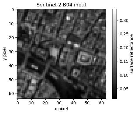
The Zarr store contains Sentinel-2 red-band reflectance (b04), projected
coordinates, longitude, latitude, CRS metadata, and source provenance. We keep
the central 64 × 64 pixels to make every method fast enough for a laptop.
dataset = xr.open_zarr(SCENE_STORE, consolidated=True)
band = dataset["b04"]

crop_size = 64
y0 = (band.sizes["y"] - crop_size) // 2
x0 = (band.sizes["x"] - crop_size) // 2
crop = band.isel(y=slice(y0, y0 + crop_size), x=slice(x0, x0 + crop_size)).load()

image = np.asarray(crop.values, dtype=np.float64)
lon_image = np.asarray(crop["longitude"].values, dtype=np.float64)
lat_image = np.asarray(crop["latitude"].values, dtype=np.float64)
valid = np.isfinite(image) & np.isfinite(lon_image) & np.isfinite(lat_image)

values = image[valid]
lon = lon_image[valid]
lat = lat_image[valid]

print(dataset)
print(f"Tutorial samples: {values.size:,}")
print(f"Reflectance range: {values.min():.4f} to {values.max():.4f}")
print("Source product:", dataset.attrs.get("source_item_id", "recorded in Zarr metadata"))
<xarray.Dataset> Size: 2MB
Dimensions:      (y: 256, x: 256)
Coordinates:
  * y            (y) float32 1kB 5.413e+06 5.413e+06 ... 5.41e+06 5.41e+06
  * x            (x) float32 1kB 4.512e+05 4.512e+05 ... 4.537e+05 4.538e+05
    latitude     (y, x) float64 524kB dask.array<chunksize=(128, 256), meta=np.ndarray>
    longitude    (y, x) float64 524kB dask.array<chunksize=(128, 256), meta=np.ndarray>
    spatial_ref  int64 8B 0
Data variables:
    b04          (y, x) float64 524kB dask.array<chunksize=(256, 256), meta=np.ndarray>
Attributes:
    other_metadata:        {'aot_retrieval_model': 'SEN2COR_DDV', 'band_descr...
    processing_history:    {'Level-0 Product': [{'facility': 'ESA', 'inputs':...
    source_cloud_cover:    0.00289
    source_collection:     sentinel-2-l2a
    source_datetime:       2026-05-27T10:56:19.024000Z
    source_item_id:        S2B_MSIL2A_20260527T105619_N0512_R094_T31UDQ_20260...
    source_stac_endpoint:  https://stac.core.eopf.eodc.eu
    stac_discovery:        {'assets': {'aod1240': {'href': '/conditions/meteo...
Tutorial samples: 4,096
Reflectance range: 0.0141 to 0.3413
Source product: S2B_MSIL2A_20260527T105619_N0512_R094_T31UDQ_20260527T133135
fig, ax = plt.subplots(figsize=(5, 4))
im = ax.imshow(image, cmap="gray", origin="upper")
ax.set(title="Sentinel-2 B04 input", xlabel="x pixel", ylabel="y pixel")
fig.colorbar(im, ax=ax, label="surface reflectance")
fig.tight_layout()
4. The common API#
Most resamplers follow the same pattern:
operator = SomeResampler(lon_deg=lon, lat_deg=lat, level=level)
result = operator.resample(values)
Building the operator determines the geometry and is usually the expensive
step. Reuse it for every band or time step sharing the same coordinates.
result.cell_ids identifies the retained NESTED HEALPix cells and
result.cell_data contains their values.
KNeighborsResampler is the shared infrastructure behind several methods,
rather than an additional end-user interpolation rule; use one of its concrete subclasses below.
At level 20 the target cells are comparable to the 10 m Sentinel-2 sampling.
LEVEL = 20
DEVICE = "cpu"


def as_numpy(array):
    if isinstance(array, torch.Tensor):
        return array.detach().cpu().numpy()
    return np.asarray(array)


def reconstruction_mse(operator, result):
    reconstructed = as_numpy(operator.invert(result.cell_data))
    return float(np.mean((reconstructed - values) ** 2))


operators = {}
results = {}
summary = []


def record(name, operator, result, *, supports_inverse=True, meaning=""):
    operators[name] = operator
    results[name] = result
    summary.append({
        "method": name,
        "output_cells": len(result.cell_ids),
        "reconstruction_mse": reconstruction_mse(operator, result) if supports_inverse else np.nan,
        "meaning": meaning,
    })
    print(f"{name}: {len(result.cell_ids):,} output cells")
Nearest neighbour#
Copies the closest observation to each output cell. It is fast, predictable, and preserves observed values, but boundaries can look blocky. It is a useful baseline and a good choice when inventing intermediate values is undesirable.
nearest = NearestResampler(
    lon_deg=lon, lat_deg=lat, level=LEVEL, device=DEVICE, verbose=False
)
nearest_result = nearest.resample(values)
record("Nearest", nearest, nearest_result, meaning="closest observed sample")
Nearest: 10,688 output cells
Bilinear interpolation#
Blends the four nearest observations with distance-based weights. It is a strong general-purpose default for continuous fields: smoother than nearest, non-iterative, and inexpensive.
bilinear = BilinearResampler(
    lon_deg=lon, lat_deg=lat, level=LEVEL, device=DEVICE, verbose=False
)
bilinear_result = bilinear.resample(values)
record("Bilinear", bilinear, bilinear_result, meaning="four-neighbour interpolation")
Bilinear: 10,559 output cells
/home/jovyan/healpix-resample/healpix_resample/bilinear.py:120: UserWarning: Sparse CSR tensor support is in beta state. If you miss a functionality in the sparse tensor support, please submit a feature request to https://github.com/pytorch/pytorch/issues. (Triggered internally at /home/conda/feedstock_root/build_artifacts/libtorch_1780240370028/work/aten/src/ATen/SparseCsrTensorImpl.cpp:49.)
  self.M  = M_coo.to_sparse_csr()
Bicubic interpolation#
Uses a radial cubic-convolution kernel and sixteen neighbours. It can retain more local curvature than bilinear, at a higher construction cost, and remains non-iterative.
bicubic = BicubicResampler(
    lon_deg=lon, lat_deg=lat, level=LEVEL, device=DEVICE, verbose=False
)
bicubic_result = bicubic.resample(values)
record("Bicubic", bicubic, bicubic_result, meaning="sixteen-neighbour cubic kernel")
Bicubic: 10,688 output cells
Clough–Tocher interpolation#
Builds a Delaunay triangulation in a local tangent plane and evaluates a
smooth, continuously differentiable bivariate interpolant. It does not
extrapolate beyond the sample convex hull and currently has no invert().
Use it for smooth regional fields when a genuine two-dimensional interpolant
is more important than operator inversion.
clough_tocher = CloughTocherResampler(
    lon_deg=lon, lat_deg=lat, level=LEVEL, device=DEVICE, verbose=False
)
clough_tocher_result = clough_tocher.resample(values)
record(
    "Clough-Tocher", clough_tocher, clough_tocher_result,
    supports_inverse=False, meaning="C1 triangulation-based interpolation",
)
Clough-Tocher: 10,275 output cells
PSF-aware reconstruction#
Treats each input pixel as a spatial measurement with a point-spread function
and solves a damped inverse problem. This is the appropriate method when the
sensor footprint matters or when reconstructing spatial scales close to the
sampling limit. lam stabilizes noise amplification; it is not needed by the
fixed interpolation methods above.
FWHM_M = 12.5
scale_m = fwhm_to_scale(FWHM_M)
npt = recommend_npt(scale_m, LEVEL, target_mass=0.99)["npt"]

psf = PSFResampler(
    lon_deg=lon,
    lat_deg=lat,
    level=LEVEL,
    sigma_m=scale_m,
    Npt=npt,
    threshold=0.1,
    device=DEVICE,
    verbose=False,
)
psf_result = psf.resample(values, lam=1e-3, max_iter=14)
record("PSF-aware", psf, psf_result, meaning="regularized sensor-footprint inversion")
print(f"FWHM={FWHM_M} m, internal scale={scale_m:.3f} m, Npt={npt}")
PSF-aware: 11,075 output cells
FWHM=12.5 m, internal scale=10.617 m, Npt=22
Group-by-cell aggregation#
Assigns each observation to its containing HEALPix cell and reduces samples
within each cell. Choose mean, sum, amin, amax, or prod. Unlike an
interpolator, it never spreads one sample over neighbouring cells.
grouped = GroupByResampler(
    lon_deg=lon, lat_deg=lat, level=LEVEL, reduce="mean", device=DEVICE, verbose=False
)
grouped_result = grouped.resample(values)
record("GroupBy mean", grouped, grouped_result, meaning="mean of samples inside each cell")
GroupBy mean: 4,096 output cells
5. Compare the continuous-field methods#
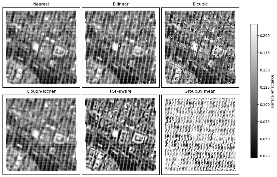
The plots show values at the actual HEALPix cell centres. The MSE column is computed after applying each operator’s reverse projection to the original sample positions; it is a diagnostic of round-trip consistency, not a claim that one method is universally best.
summary_table = pd.DataFrame(summary)
summary_table
| method | output_cells | reconstruction_mse | meaning | |
|---|---|---|---|---|
| 0 | Nearest | 10688 | 2.456783e-36 | closest observed sample |
| 1 | Bilinear | 10559 | 3.325749e-05 | four-neighbour interpolation |
| 2 | Bicubic | 10688 | 3.986735e-02 | sixteen-neighbour cubic kernel |
| 3 | Clough-Tocher | 10275 | NaN | C1 triangulation-based interpolation |
| 4 | PSF-aware | 11075 | 1.055560e-08 | regularized sensor-footprint inversion |
| 5 | GroupBy mean | 4096 | 0.000000e+00 | mean of samples inside each cell |
def plot_healpix_result(ax, name):
    result = results[name]
    cell_lon, cell_lat = hp.healpix_to_lonlat(
        as_numpy(result.cell_ids), LEVEL, ellipsoid="WGS84"
    )
    scatter = ax.scatter(
        cell_lon, cell_lat, c=as_numpy(result.cell_data),
        s=5, cmap="gray", vmin=np.nanpercentile(values, 1),
        vmax=np.nanpercentile(values, 99), linewidths=0,
    )
    ax.set_title(name)
    ax.set_xticks([])
    ax.set_yticks([])
    return scatter


names = ["Nearest", "Bilinear", "Bicubic", "Clough-Tocher", "PSF-aware", "GroupBy mean"]
fig, axes = plt.subplots(2, 3, figsize=(11, 7), constrained_layout=True)
for ax, name in zip(axes.flat, names):
    scatter = plot_healpix_result(ax, name)
fig.colorbar(scatter, ax=axes, label="surface reflectance", shrink=0.8)
<matplotlib.colorbar.Colorbar at 0x734e185ddf90>
6. Conservation is a different objective#
ConservativeResampler is for integrated quantities. It bins each sample into
its containing cell and preserves sum(value × source area). Its output is an
amount per cell, so it should not be compared visually with interpolated
reflectance values.
If the input already stores an extensive amount, omit area (equivalent to an
area of one). Here reflectance is treated only as a convenient numerical
example with 10 m × 10 m source footprints.
source_area_m2 = np.full(values.shape, 10.0 * 10.0)
conservative = ConservativeResampler(
    lon_deg=lon,
    lat_deg=lat,
    level=LEVEL,
    area=source_area_m2,
    device=DEVICE,
    verbose=False,
)
conservative_result = conservative.resample(values)

integral_in = float(np.sum(values * source_area_m2))
integral_out = float(np.sum(as_numpy(conservative_result.cell_data)))
print(f"Input integral:  {integral_in:.12g}")
print(f"Output integral: {integral_out:.12g}")
print(f"Relative error:  {abs(integral_out - integral_in) / abs(integral_in):.3e}")
Input integral:  38470.48
Output integral: 38470.48
Relative error:  1.891e-16
7. Exact point indexing#
CellPointResampler stores each coordinate in a fixed level-29 cell, which is
small enough to act as a point identifier. It is useful for indexing and
joining observations, not for producing a smooth raster.
cell_points = CellPointResampler(
    lon_deg=lon, lat_deg=lat, reduce="mean", device=DEVICE, verbose=False
)
cell_point_result = cell_points.resample(values)
roundtrip = as_numpy(cell_points.invert(cell_point_result.cell_data))
print(f"Input points: {values.size:,}")
print(f"Level-29 cell-points: {len(cell_point_result.cell_ids):,}")
print(f"Maximum round-trip error: {np.max(np.abs(roundtrip - values)):.3e}")
Input points: 4,096
Level-29 cell-points: 4,096
Maximum round-trip error: 0.000e+00
8. Discrete data: categories versus independent bits#
Continuous interpolation is not appropriate for integer labels.
CategoricalResamplertreats values as mutually exclusive classes and selects the strongest class in each cell.BitmaskResamplertreats every bit as an independent flag, resamples each flag separately, and recombines the output bits.
The simple labels below are derived from the real reflectance only to keep the tutorial self-contained.
q1, q2 = np.quantile(values, [1 / 3, 2 / 3])
land_cover = np.digitize(values, [q1, q2]).astype(np.int64)

categorical = CategoricalResampler(
    lon_deg=lon, lat_deg=lat, level=LEVEL, device=DEVICE, verbose=False
)
categorical_result = categorical.resample(land_cover, return_scores=True)
print("Input classes:", np.unique(land_cover))
print("Output classes:", np.unique(as_numpy(categorical_result.cell_data)))
print("Score array shape:", as_numpy(categorical_result.scores).shape)
Input classes: [0 1 2]
Output classes: [0 1 2]
Score array shape: (3, 10559)
bright = (values > np.median(values)).astype(np.int64)       # bit 0
northern = (lat > np.median(lat)).astype(np.int64)         # bit 1
quality_flags = bright | (northern << 1)

bitmask = BitmaskResampler(
    lon_deg=lon, lat_deg=lat, level=LEVEL, n_bits=2,
    device=DEVICE, verbose=False,
)
bitmask_result = bitmask.resample(quality_flags)
print("Input bitmasks:", np.unique(quality_flags))
print("Output bitmasks:", np.unique(as_numpy(bitmask_result.cell_data)))
Input bitmasks: [0 1 2 3]
Output bitmasks: [0 1 2 3]
9. Choosing a resampler#
Need |
Recommended starting point |
|---|---|
Fast baseline; do not invent new values |
|
General continuous field |
|
More local curvature, fixed non-iterative kernel |
|
Smooth regional bivariate interpolation |
|
Known sensor footprint or inverse reconstruction |
|
Mean, sum, minimum, or maximum inside each cell |
|
Preserve an integrated amount |
|
Treat coordinates as exact point identifiers |
|
One mutually exclusive label per sample |
|
Independent flags packed into bits |
|
The important question is therefore not “which interpolation has the smallest number in this example?” but “what quantity should the output cell represent?” Once that estimand is clear, the table above usually narrows the choice to one or two methods.
For detailed parameters and mathematical definitions, continue with the user guide and the API reference.