HEALPix → UTM: extract a small UTM zone from a large HEALPix dataset#
This notebook shows how to convert data stored on HEALPix cells — cell_ids and data[B, N], where B is a batch
dimension (bands, time steps, …) — into a regular raster x, y in the UTM projection of a tile.
The important point is the order of operations. A metre-scale HEALPix dataset covering the Earth is far larger than memory (terabytes to petabytes in a Zarr store), so the data can never be loaded first. Instead:
describe the target: the
x,ypixel centres of the zone and the CRS of the tile;build the operator from that geometry only — this tells us which HEALPix cells are needed;
read only those cells from the store;
apply the operator to the data that were read.
Steps 1–2 never touch the dataset: their cost depends on the size of the raster, not on the size of the archive.
Requirements: healpix-resample with the optional pyproj dependency (pip install healpix-resample[utm]), and
matplotlib for the figures.
import warnings

import numpy as np
import matplotlib.pyplot as plt
import healpix_geo

# torch emits informational warnings about its sparse-tensor backend
warnings.filterwarnings("ignore", message=".*[Ss]parse.*")

from healpix_resample import HealpixToUTM, UTMGrid
The source dataset#
To keep the notebook self-contained (no download), the “store” below is a function that returns the values of
any requested cells, computed analytically. It stands for a selection in a real Zarr store (see
the last section, With a real Zarr store); what matters is its interface: cell ids in, data[B, K] out.
The dataset is global at HEALPix level 19 (cells of about 12 m), with B = 3 fields. It is never materialised.
LEVEL = 19                 # HEALPix level of the dataset (nested scheme)
B = 3                      # batch dimension: bands, dates, ...
WAVELENGTHS_M = (400.0, 700.0, 1200.0)
R = 6371000.0

n_cells_global = 12 * 4**LEVEL
cell_size_m = np.sqrt(4 * np.pi / n_cells_global) * R
print(f"global dataset: {n_cells_global:.2e} cells of ~{cell_size_m:.1f} m, "
      f"{B * n_cells_global * 4 / 1e12:.0f} TB as float32")


def field(lon_deg, lat_deg):
    """The 'true' geophysical fields, defined everywhere: shape (B,) + lon.shape."""
    lon_deg = (np.asarray(lon_deg) + 180.0) % 360.0 - 180.0   # same convention for [0, 360) and [-180, 180)
    xm = R * np.radians(lon_deg) * np.cos(np.radians(48.3))
    ym = R * np.radians(lat_deg)
    return np.stack([np.sin(2 * np.pi * xm / w) * np.cos(2 * np.pi * ym / w) for w in WAVELENGTHS_M])


def read_cells(cell_ids):
    """Stand-in for the store: return data[B, K] for the requested cell ids only."""
    lon, lat = healpix_geo.nested.healpix_to_lonlat(
        np.asarray(cell_ids, dtype=np.uint64), LEVEL, ellipsoid="WGS84"
    )
    return field(np.asarray(lon), np.asarray(lat)).astype(np.float32)
global dataset: 3.30e+12 cells of ~12.4 m, 40 TB as float32
1. The target zone: x, y and the reference of the tile#
The zone is described by the pixel-centre coordinates x (eastings) and y (northings) and by the CRS of the
tile they belong to. Here: a 2 km × 2 km zone at 10 m in UTM zone 30N (EPSG:32630), the projection of the
Sentinel-2 tiles over Brittany. y is decreasing (north-up raster).
TILE_EPSG = 32630          # CRS of the tile (WGS 84 / UTM zone 30N)
RES = 10.0                 # pixel size (m)

x = 400000.0 + RES * (np.arange(200) + 0.5)     # (nx,) pixel centres
y = 5360000.0 - RES * (np.arange(200) + 0.5)    # (ny,) pixel centres, north-up

grid = UTMGrid(crs=TILE_EPSG, x=x, y=y)
print("raster shape (ny, nx):", grid.shape, "|", grid.crs.name)
raster shape (ny, nx): (200, 200) | WGS 84 / UTM zone 30N
UTMGrid.from_bounds(crs, (xmin, ymin, xmax, ymax), resolution) builds the same object from the outer edges
of the zone.
2. Build the operator: which cells are needed?#
HealpixToUTM is built from the grid and the HEALPix level only. Internally it reprojects the pixel centres to
longitude/latitude, builds a resampler on those points, and will later apply that resampler’s invert()
(HEALPix cells → points). Building the resampler is what determines the cells the raster depends on, exposed
as op.cell_ids (sorted, unique).
op = HealpixToUTM(grid, LEVEL, method="bilinear")

print(f"cells needed: K = {op.K}")
print(f"fraction of the global dataset: {op.K / n_cells_global:.1e}")
print("first ids:", op.cell_ids[:4])
cells needed: K = 26353
fraction of the global dataset: 8.0e-09
first ids: [925142264303 925142264307 925142264312 925142264313]
3. Read only those cells#
This is the only access to the dataset, and it is limited to K cells.
data = read_cells(op.cell_ids)
print("data:", data.shape, data.dtype, f"({data.nbytes / 1e6:.2f} MB)")
data: (3, 26353) float32 (0.32 MB)
4. Apply the operator#
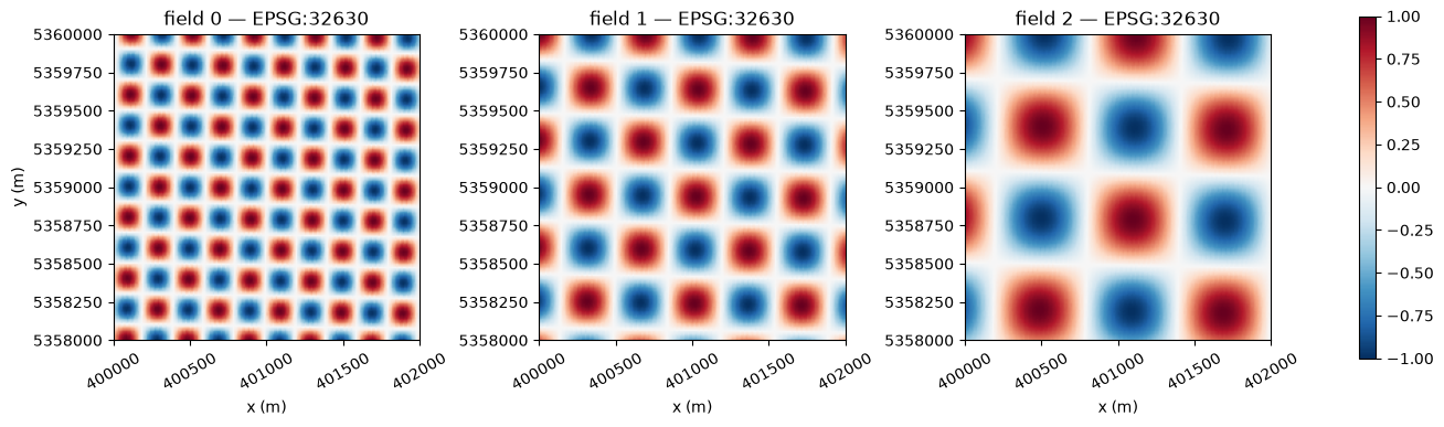
resample takes data[B, K] (or a single field data[K]) and returns image[B, ny, nx]. The operator can be
reused for any other data defined on the same cells — other dates, other variables — without being rebuilt.
image = op.resample(data)
print("image:", image.shape, image.dtype)
image: (3, 200, 200) float64
extent = [grid.x[0] - RES / 2, grid.x[-1] + RES / 2, grid.y[-1] - RES / 2, grid.y[0] + RES / 2]

fig, axes = plt.subplots(1, B, figsize=(13, 4.2), constrained_layout=True)
for b, ax in enumerate(axes):
    im = ax.imshow(image[b], extent=extent, origin="upper", vmin=-1, vmax=1, cmap="RdBu_r")
    ax.set_title(f"field {b} — EPSG:{TILE_EPSG}")
    ax.set_xlabel("x (m)")
    ax.ticklabel_format(style="plain", useOffset=False)
    ax.tick_params(axis="x", labelrotation=30)
axes[0].set_ylabel("y (m)")
fig.colorbar(im, ax=axes, shrink=0.8)
plt.show()
Choosing the interpolation method#
method selects which resampler’s invert() is used. Since the test field is analytic, the result can be
compared with the truth at the pixel centres. Each method needs a slightly different set of cells, so the read
is repeated with each operator’s own cell_ids.
lon_pix, lat_pix = grid.lonlat()
truth = field(lon_pix, lat_pix)

print(f"{'method':<15}{'K':>8}{'rms error':>12}{'max error':>12}")
for method in ["nearest", "bilinear", "bicubic", "clough_tocher"]:
    op_m = HealpixToUTM(grid, LEVEL, method=method)
    err = op_m.resample(read_cells(op_m.cell_ids)) - truth
    print(f"{method:<15}{op_m.K:>8}{np.sqrt(np.nanmean(err**2)):>12.1e}{np.nanmax(np.abs(err)):>12.1e}")
method                K   rms error   max error
nearest           25987     3.2e-02     1.6e-01
bilinear 26353 9.9e-03 5.4e-02
bicubic 26378 1.0e-02 7.5e-02
clough_tocher 27195 9.4e-05 3.8e-04
"nearest": each pixel takes the value of the cell that contains it. Use it for categorical data and masks."bilinear"(default) and"bicubic": weighted averages of the 4 / 16 nearest cells. They smooth slightly."clough_tocher": Delaunay triangulation of the cell centres and a C1 cubic interpolant. The most accurate on smooth fields; slightly more cells and a longer construction.
The errors above are relative to a field of amplitude 1 whose shortest wavelength (400 m) is sampled by 12 m cells; they are not a general accuracy statement.
Missing data#
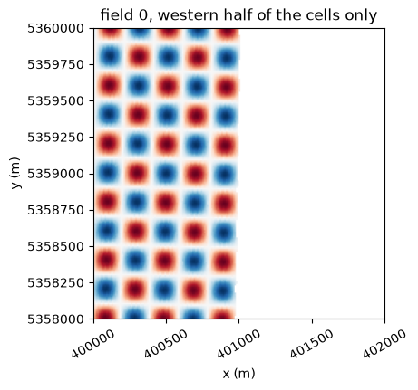
A pixel that depends on a cell without data is returned as NaN — nothing is extrapolated. This applies both
to NaN values in data and to cells that are absent from the store. In the second case, pass the ids of the
cells that were actually read with cell_ids=; they can be in any order.
# Suppose the store only holds the western part of the zone.
lon_c, _ = healpix_geo.nested.healpix_to_lonlat(op.cell_ids.astype(np.uint64), LEVEL, ellipsoid="WGS84")
lon_c = (np.asarray(lon_c) + 180.0) % 360.0 - 180.0
available = op.cell_ids[lon_c < np.median(lon_c)]

partial = op.resample(read_cells(available), cell_ids=available)
print(f"pixels with a value: {np.isfinite(partial[0]).mean():.0%}")

fig, ax = plt.subplots(figsize=(4.6, 4.2), constrained_layout=True)
ax.imshow(partial[0], extent=extent, origin="upper", vmin=-1, vmax=1, cmap="RdBu_r")
ax.set_title("field 0, western half of the cells only")
ax.set_xlabel("x (m)"); ax.set_ylabel("y (m)")
ax.ticklabel_format(style="plain", useOffset=False)
ax.tick_params(axis="x", labelrotation=30)
plt.show()
pixels with a value: 50%
With a real Zarr store#
With xarray, step 3 becomes a lazy selection: only the chunks that contain the requested cells are read.
The pattern below is not executed here; adapt the names of the dimension and of the variables to your store.
import xarray as xr

ds = xr.open_zarr("s3://bucket/dataset.zarr")        # lazy: nothing is read yet
level = ds.cell_ids.attrs["level"]                   # or the known level of the store

op = HealpixToUTM(grid, level, method="bilinear")    # geometry only

# (a) sparse store: `cell_ids` is an indexed coordinate
sub = ds.sel(cell_ids=op.cell_ids)

# (b) full-sphere store in nested order: the position along the dimension *is* the cell id
sub = ds.isel(cells=op.cell_ids)

data = sub["reflectance"].transpose(..., "cells").values     # (B, K): the only read
image = op.resample(data)                                    # (B, ny, nx)

out = xr.DataArray(
    image, dims=("band", "y", "x"),
    coords={"y": grid.y, "x": grid.x},
    attrs={"crs": grid.crs.to_wkt()},
)
Notes:
op.cell_idsis sorted, so the selection reads each chunk at most once.If some required cells are missing from a sparse store, select the ones that exist (
np.intersect1d(op.cell_ids, ds.cell_ids)) and pass them toop.resample(data, cell_ids=...).For a ring-ordered store, build the operator with
nest=False.For a large zone, process it tile by tile: one operator per tile keeps
K, and therefore the read, bounded.device="cuda"builds and applies the operator on GPU;dtype=torch.float32halves its memory.